Workflow
In this part, we will show you all the steps we did to obtain all our final results including Time series analysis and potential source analysis.
Step1 Data Collection
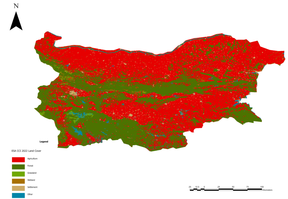
• Download CAMS NetCDF datasets for NO₂ and PM2.5 (2013–2022) • Retrieve WorldPop 2020 population raster • Acquire GAUL Level-2 administrative boundaries • Obtain ESA CCI Land Cover raster (2013-2022)
Special Steps
Firstly, according to the experimental requirements, the Bulgarian vectors were extracted by downloading CAMS NetCDF datasets for NO₂ and PM2.5, Retrieve WorldPop 2020 population raster, Acquire GAUL Level-2 administrative boundaries, Obtain ESA CCI Land Cover 2022 raster. Then process CAMS NetCDF data to supplement the December 2022 summary into monthly raster maps.
Step2 Data Preprocessing
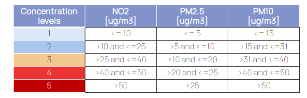
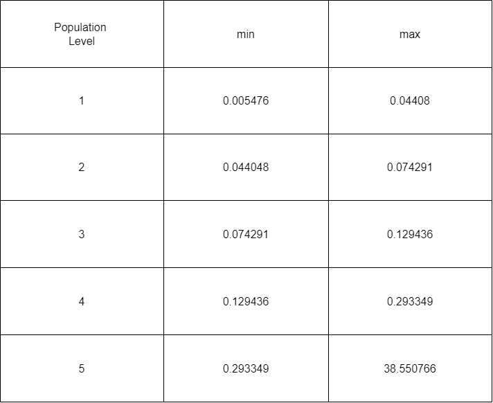
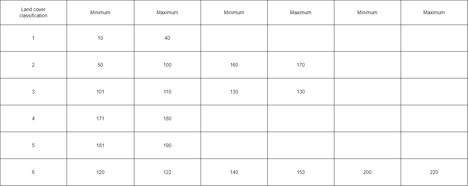
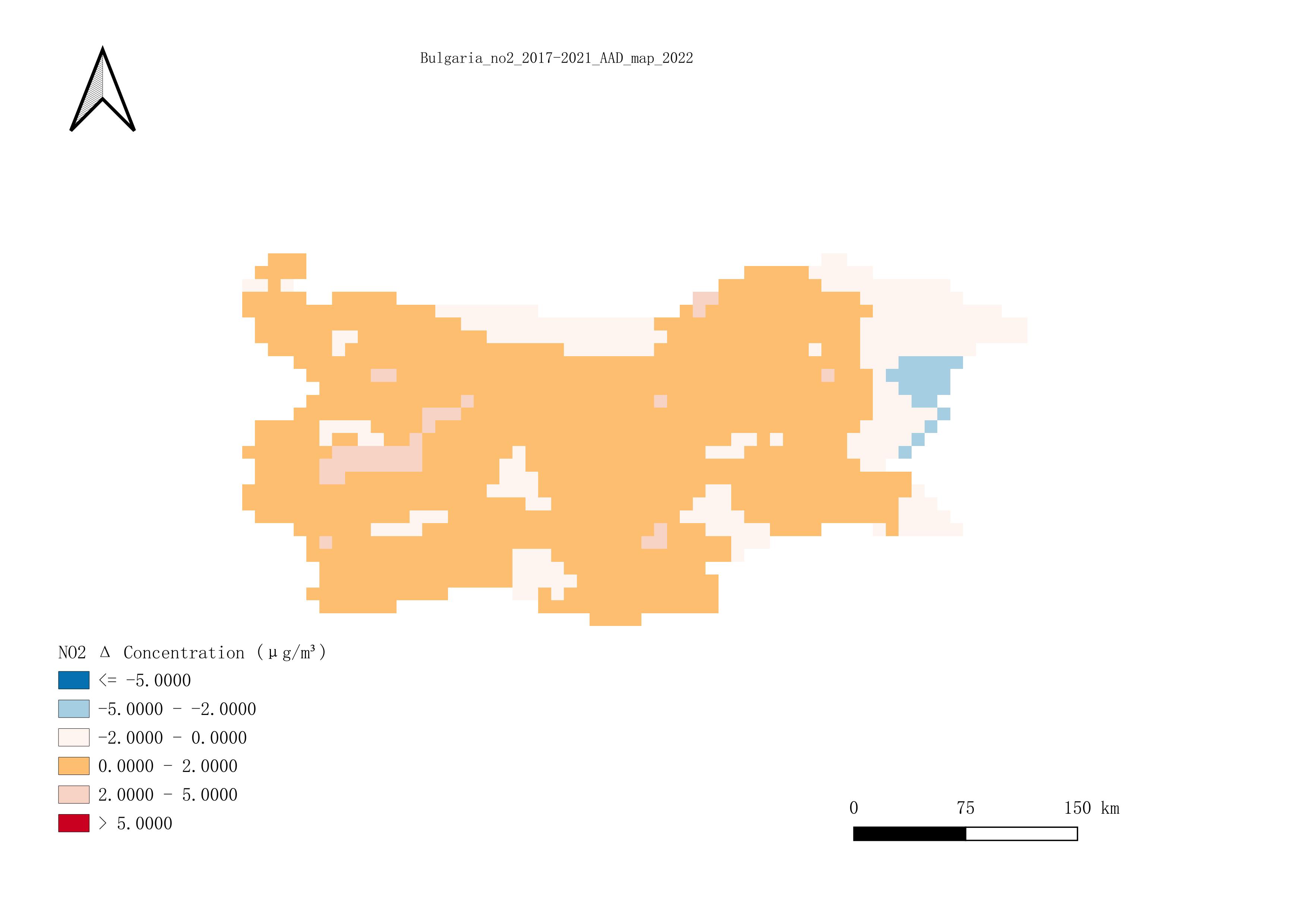
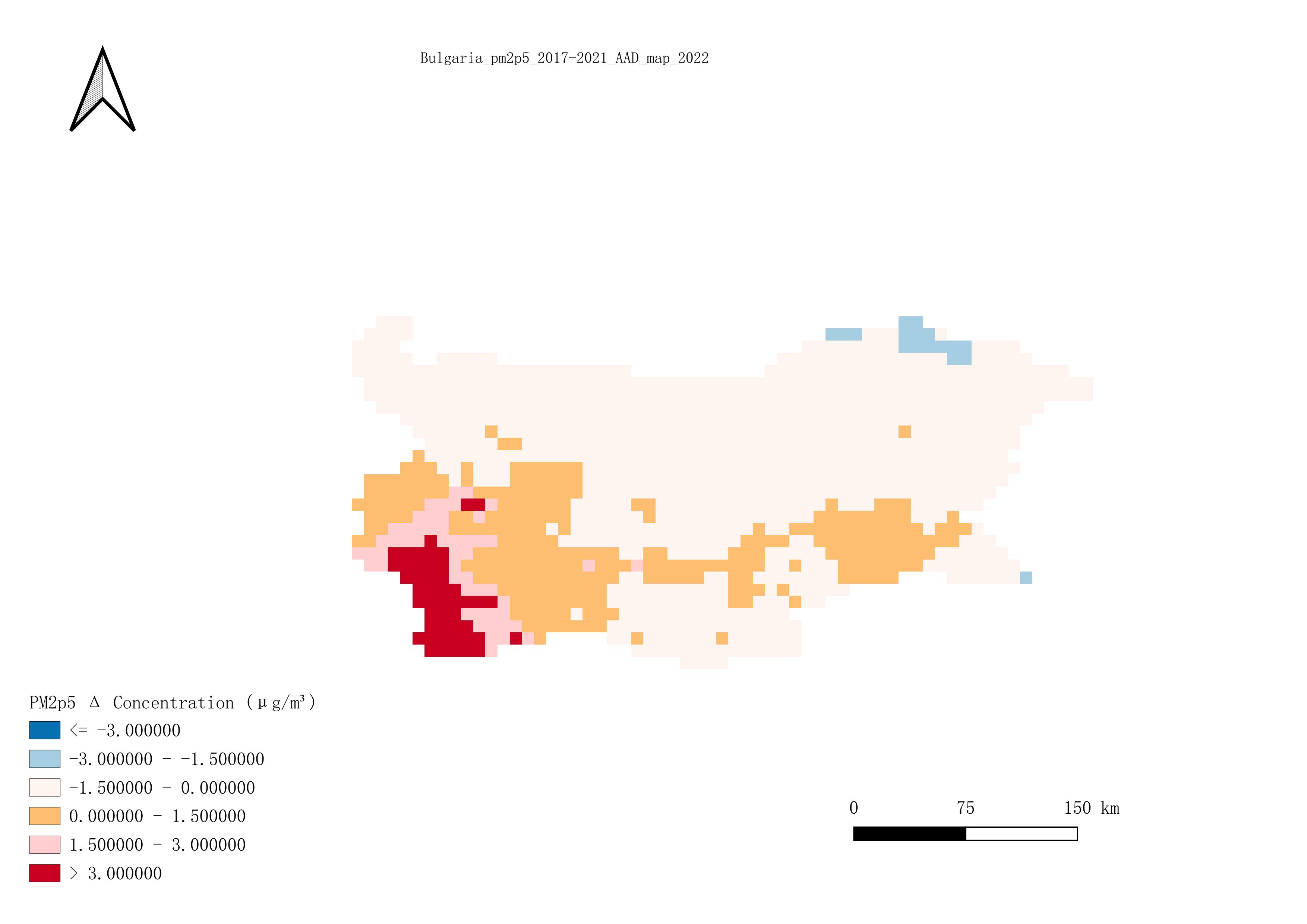
• Clip all rasters to the national boundary of Bulgaria • population raster into five classes • Reclassify pollutant concentration into five risk levels • Simplification of the ESA CCI Land Cover 2013-2022 raster based on the IPCC generic model • Convert monthly/annual NetCDF data into raster layers • Calculation of a plot of the difference between a calendar year and its average over the previous five years
Special Steps
First, we used QGIS to summarize the processed monthly data and calculate annual and seasonal averages. To analyze inter-annual as well as seasonal variations in pollutants. Then, We then reclassify population, pollutant concentration, and land cover according to the relevant norms
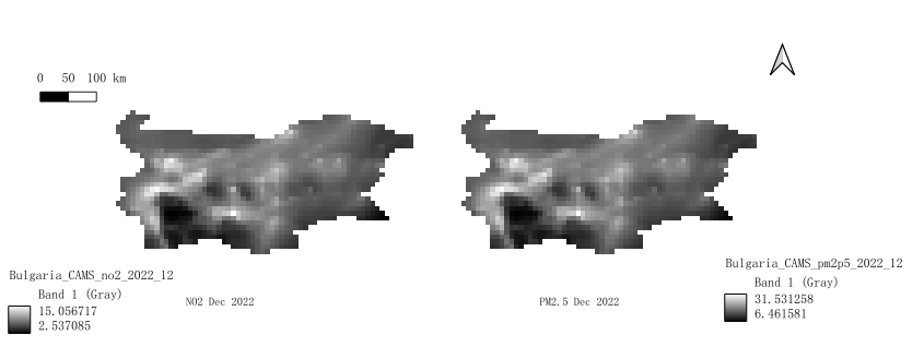
Next, we compute difference maps comparing 2022 with the 2017-2021 average to analyze the deviation of air quality from the recent historical average.
Take care to ensure consistency in the data to ensure that the data are at the same resolution, Lets resample the CAMS (Average pollutant maps all years) to match the ESA LC product.
step3 Land Cover-Based Exposure Analysis
• Convert ESA CCI 2022 land cover raster to vector polygons • Retain only the "Settlement/Urban" land cover class • Dissolve urban polygons into a single geometry • Use the dissolved urban mask to extract average and maximum pollutant exposure via zonal statistics
Special Steps
We convert only the built-up areas to vectors and perform partition statistics (zoning statistics) on them. Then we used the layer Joins to add Min and Max for all years 2013-2022.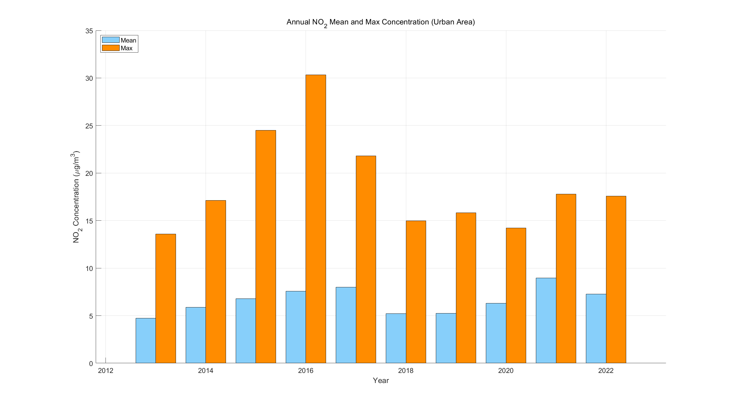
Step4 Zonal Statistics
• Compute zonal population class median per administrative unit • Extract maximum pollutant values per unit using zonal statistics • Combine population and pollution data to generate a bivariate exposure indicator
Special Steps
First, we use QGIS, in quantile mode, to divide the data into five classes such that each class contains the same number of features or pixels, regardless of the actual range of values. Then, we use the Bulgarian GAUL L2 data to calculate raster statistics for pollutants and population. Then to reveal spatial patterns of interactions and to explore heavily polluted and densely populated areas, we define the \(bivariate=pollutant class max*10+population class median\).
Step5 Highlight
• Time Series Analysis Data used in this analysis are derived from CAMS (Copernicus Atmosphere Monitoring Service) NetCDF datasets.
Hourly pollutant concentrations of PM2.5 and NO₂ were extracted for December (2013–2022) using QGIS mesh tools.
One point was selected from a densely urbanized area where pollutant concentrations were relatively high in the annual average distribution. This point was used as a representative location for time-series extraction.
The values at 00:00 and 12:00 were exported and visualized using MATLAB. • potential source analysis Based on the Global Data Assimilation System Reanalysis of Meteorological Data (GDAS), the backward trajectory model of HYSPLIT was used to simulate the backward trajectory of the air 500m above sofia from December 2022, and the spatial similarity of the trajectories was further computed by applying the angular distance function so as to cluster the trajectories. The direction of the possible sources of pollutants was thus analyzed. The generated maps (e.g., land cover reclassification maps, binary exposure maps combining population and contamination risk, pie charts summarizing population distribution by exposure class, etc.) can be found on the visible page Results and WebGIS .